“The spirit that interferes with (the development of masculinity in boys) … negates consciousness. It’s antihuman, desirous of failure, jealous, resentful, and destructive. No one truly on the side of humanity would ally him or herself with such a thing. No one aiming at moving up would allow him or herself to become possessed by such a thing. And if you think tough men are dangerous, wait until you see what weak men are capable of.”

Jordan Peterson

Code can be found here.

Motivation

In 12 Rules for Life, clinical psychologist Jordan Peterson, someone I look up to greatly as he has exposed me to copious amounts of wisdom and direction, abashes unmasculine men. He demands men to toughen up, be independent, be assertive, and aggressive. He argues that harassment between men is normal for acceptance, and men who do not gracefully participate are narcissists. Modern society is criticized for being judges of the natural hierarchy, actions that will surely come bite itself when it results in “harsh, fascist political ideology” as lackluster masses garner an unconscious fascination with any leadership.

Unraveling Peterson’s arguments also meant the reflection of my life. I had associated phrases such as “toughen up! Be a man!” as nothing more than conservative talk. I had decided that gender roles weren’t all that important in life. To be caring, compassionate, sensitive to others were what mattered. This proved to be in stark contrast to what I was reading, which shattered my suppositions. Had I been approaching life all wrong?

I became fascinated by the topic of masculinity from all prespectives. I watched shorts such as “DICKS - Do you need one to be successful” and opinions pieces, such as this one from The Atlantic on a father’s reaction to society and his experiences while raising a gender creative son. I’m reading books such as “No More Mr. Nice Guy” and “The Way of the Superior Man”, for direction. Often, I questioned why I was doing all this, and if I should stop and just “be myself” and let the obsession slide. However, I even more strongly believed that covering everything in veils of ignorance does not bring justice to one’s life.*

Reviewing this days after the first draft has made me appreciate how useful it was to look at the subject from multiple opinions.

In my obsession, I found this article from FiveThirtyEight, a fascinating website that uses statistics to tell stories. In it, over a thousand men were surveyed on their thoughts of masculinity. This seemed like data that I wanted to play with, and a way to learn some ML skills in the process. I found the data on Kaggle and got to work.

Data Form

The survey composed of 1189 participant responses, from a 30-question survey who’s PDF form can be found here. The survey is divided split into 5 parts: The first being views on masculinity in general, the second being lifestyle choices, third being views on masculinity and employment, particularly the #metoo movement, fourth on relationships, and lastly a section on demographics. Although there were some open-ended questions in the survey, these were not supplied in the dataset.

I loaded up pandas on Jupyter Notebook, and got to work!

Thinking of a Question

For brevity, ‘masculine’ will be shorthanded to M, and non-masculine will be shorthanded to NM.

I was interested in the differences in men who approached life with different levels of masculinity. Many of the survey questions, such as “Have you seen of a sexual harassment incident at work.”, did not have a clear answer of what deemed as M or NM. The feature columns ultimately decided to use in my analysis were the answers to the following:

• In general, how masculine or “manly” do you feel?
• How important is it to you that others see you as masculine?
• How often do you ask a friend for personal advice? *
• How often do you express physical affection to male friends, like hugging, rubbing shoulders? *
• How often do you cry? *
• How often do you have sexual relations with women?
• How often do you have sexual relations with men? *
• How often do you see a therapist? *
• How often do you feel lonely or isolated? *
• How often do you get in a physical fight?
• How often do you watch sports?
• How often do you work out?

‘*’ represents NM qualities.

Looking through the survey, the label spoke out to me: What is your sexual orientation? That seemed interesting! Hence, my question became: Could we use masculinity as a predictor of sexual orientation?

Cleaning the Data

Mapping the Data

The responses to the question were given in string form, such as “Very masculine”, “Somewhat masculine.”. These responses must first be mapped to numbers. As Q1Q2 were on a 4 point scale, I mapped those responses to [0,3], and to [0,4] for the rest of the questions. I wanted the bigger number to represent the more M feature, hence 0 representing the NM feature.

for column in lifestyle_cols_to_map_nomasc:
    survey[column] = survey[column].map({"Often": 0, "Sometimes": 1, "Rarely": 2, "No answer": 3, "Never, but open to it": 3, "Never, and not open to it": 4})
    
for column in lifestyle_cols_to_map_masc:
    survey[column] = survey[column].map({"Often": 4, "Sometimes": 3, "Rarely": 2, "Never, but open to it": 1, "Never, and not open to it": 0})

This was my first mistake and something I would not do in the future. Although intuitively it sounded appealing, not only does this require extra work, but it becomes quite confusing. For example, when trying to figure out which labels are weighed more in the calculation of sexual orientation, I constantly had to keep on going back to figure what a positive value meant. Did it mean it was a NM label that was never done or a M label that was often done?

As for my labels, I mapped “Straight” to 1, else 0.

Dealing with Missing Data

Another mistake occurred here. Through inspection, I concluded that missing data were labeled as ‘NaN’, something that is common for datasets. However, it was only running some algorithms, and after investigating why things did not add up did I realized that both ‘NaN‘ and the string “Not available” were used for missing data. The time I could have saved! This taught me to do a more thorough .value_counts() in the future and to make sure I understand my data before proceeding.

I also had to figure out what to do with the missing data. The first time I ran the model, not wanting to do any more reading, I opted for a quick-and-dirty dropna, which elements all rows where one of the column responses were missing. This led to 212 participants being dropped, an 18% dataset reduction. The detriment this had on my model’s accuracy compared to my second implementation was noticeable, however.

Using KNN-Imputation

Instead of removing missing features, we can fill the spaces with missing features by taking an educated guess of what that value would have been. Although common approaches are finding the average of a column, using a K Nearest Neighbor Imputation seems to be a superior method. KNN-Imputation takes in a dataframe, finds the euclidian distances of each row (whose features are converted to a vector) with one another. Any missing feature is imputed by the mean of the n nearest neighbors in terms of that distance, where n is a parameter of our choosing.

from sklearn.impute import KNNImputer

imputer = KNNImputer(n_neighbors=2)
useful_df_array = imputer.fit_transform(useful_df)

I chose n = 2 randomly. However, what can improve my model even further is running a loop testing n values from say [1,100], and then picking the n-value that resulted in the most accuracy.

Dealing with Label Imbalances

The labels for sexual orientation were “Straight”, “Bisexual”, “Gay”, “Other”. To be expected, the number of Straight data points greatly outnumbers anything else, with about 7x more labels for straight than the other responses. Hence, to deal with this difference, I would have to introduce a bias to the data to even out the labels. There are two types of data imbalance:

Oversampling: When data is even out by adding more of minority labels. Undersampling: The removal of over-represented, majority labels.

As undersampling is used when there are copious amounts of data, I did not have enough data for me to ignore. I opted to oversample the non-straight orientations. However, I could not go out and replicate the survey to non-straights, so I opted to use Synthetic Minority Oversampling Technique (SMOTE). A random minority is selected. Then, using information from n (default 5) of its nearest neighbors, a synthetic member of that minority group is created. This is repeated until the number of minority labels is equal to the number of majority labels.

Normalizing Features

Normalizing is used on features to place feature data on either the same or a similar scale. This is to account for the difference in scale that values can have. For example, if our data were movies, with features being (IMDB rating, year released), then a difference in one year in the release is insignificant in comparison to a one-point difference in IMDB rating. As a result, normalizing data is required. As 2 of the questions took place on a 4 point scale, and the rest on a 5 point scale, and because there were no outliers in the data, I opted for a simple min-max normalization, to get all feature points in [0,1]

Now that our data was cleaned, it’s time to make some predictions!

Choosing and Applying Supervised Machine Learning Models

Overwhelmed by all my possible choices, I first used K-Nearest Neighbours and Logistic Regression. They made the most intuitive sense and were the simplest for me to understand.

K-Nearest Neighbours

K-Nearest Neighbours (KNN) works by giving each piece of the testing data a point representation in length(features)-dimensional space. To find what category the new piece of data belongs to, we look up its k-nearest training data points. We count up how many of them “Straight” represented by 1, and how many are not, represented by a 0. The value with the most representation will be the value of our new data point.

To find what value of k to use, k values from 1 to 200 were tried out on the same test and training set. The accuracy values are given by the y-axis:

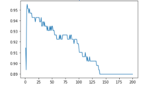
It seems like, after a peak of 3, underfitting (not using enough information from the training data) started occurring. Hence, k=3 was chosen.

To test if a model performs well or not, accuracy and F1 scores are helpful indicators. Accuracy represents how the percentage of times where the model’s predicted sexual orientation, and actual orientation was correct. Recall measures the percentage of the relevant items the classifier was able to successfully find, and precision measures the percentage of items the classifier found that was relevant. The F1 score takes into factor both the precision and the recall.

Using k=3, I went on to find the accuracy and F1 Score of my model. Because of how small the dataset was, I was afraid that just running the model on one random state of generated test and training data would be too volatile. Hence, I ran the model on 20 random states and plotted its accuracy. This is with uneven labels (before SMOTE was applied) and missing values deleted:

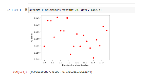
On average, based on 20 iterations, an accuracy of 93% and an F1 score of 0.96. Compared to a model that guessed ‘Straight’ all the time, that model would get 848 / (848 + 129), or an 87% accuracy.

After SMOTE-ing the data, and running on the same random states, this was the result:

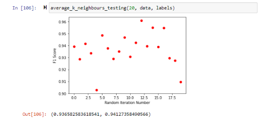
While the accuracy increased to 94%, the F1 score went down, indicating a decrease in either precision or recall or both. Despite the F1 score loss, this was a success, as accuracy was what was important here.

Logistic Regression Model

Unlike a y = mx+b linear model, a logistic model uses a Sigmoid function to provide the probability that a new value is mapped to a 0 or 1. By using a Logistic Regression Model, it gave me access to which factors had the biggest weighting in the mapping, They are as follows:

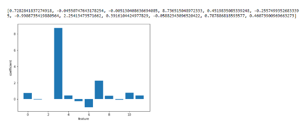
Features in reference: [“q0007_0002”, “q0007_0003”, “q0007_0004”, “q0007_0007”, “q0007_0010”, “q0007_0011”, “q0007_0005”, “q0007_0006”, “q0007_0008”, “q0007_0009”, ‘q0001’, ‘q0002’]

The interpretation of the graph is made tiring with my previous choice to map masculine traits to higher numbers, and non-masculine traits to lower numbers. The heaviest factor was associated with whether or not one had sexual relations with men. As a higher number represents more masculine (in that case), a higher coefficient for index 3 means that they DO NOT have sexual relationships when men (which makes sense, straight guys are less likely to mingle with men). This was much more of a factor than having relationships with women, with both straight and non-straight guys do. The only negative factor, crying, means that the more a man cried, the more chance of being straight he was. Once again, I wish that I had mapped all values by the same metric, but here we are.

Running the on SMOTEd data, and averaging 20 different random-state runs, resulted in 91.4 % accuracy.

It was only here I started to research what ML model would benefit me the most. I came across this cheat sheet:

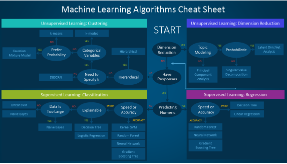
which suggested I try a Support Vector Machine algorithm. It was also at this point where I implemented KNN-Imputation.

Support Vector Machines (SVM)

At its crux, a SVM attempts to make a decision boundary. It is easily imagined when there are only 2 features, like so:

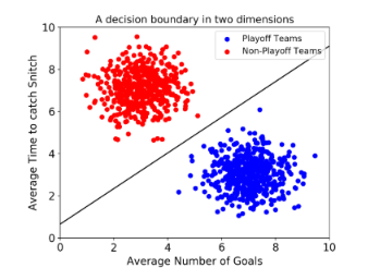
Then, when a new point is plotted, depending on where that point is plotted determines its label. Not all decision boundaries are linear. They can look like this as well:

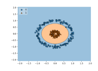
Such a mapping is produced by mapping each of the points to an n+1 dimensional space, creating a linear decision boundary, and then mapping everything back to n-dimension. However, the most often used decision boundary is made with radical bias function (rbf kernel), which can produce boundaries like this:

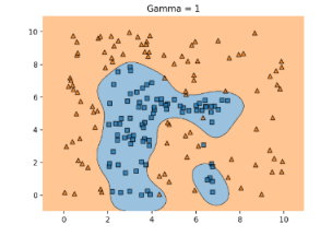
The error value, C, is how strict a boundary point is. When C is large, then SVM uses a hard margin, not allowing for misclassifications. However, it becomes very attentive to outliers. This runs the risk of overfitting. If C is too small, underfitting risk increases. In the rbf kernel, gamma is akin to the error value. To maximize accuracy, I had to find the perfect gamma value! Initializing a SVC, I found accuracy scores for Gammas in the range [0.1, 10], each score an average of 20 random-state runs:

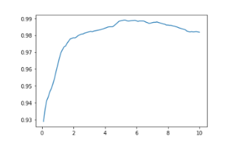
Which showed me that a Gamma of 5.2 was the sweet spot, which produced an average accuracy of 98.9% of distinguishing if a person was straight or not! Amazing! This model was much better than the previous ones!

Applying an Unsupervised Maching Learning Model

K++ Clustering

Satisfied with my model, I wondered if what the models would naturally divide the participants on, and if this division could be based around orientation? The first unsupervised ML model I knew was using K++ Clustering.

What this does is given only feature data and no labels, the data is plotted with strategically placed centroids (unlike K Clustering) with the number of centroids being how many clusters you think the data should/could divide into. Each piece of data calculates which centroid it is closest to, and becomes part of that cluster. In our case, since we are splitting the label into straight/not straight, there are 2 clusters. We repeat until convergence, and the two groups are produced.

These were the centroids of the 2 groups that converged:

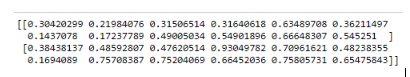
So yes! K++ did find that the groups would be separated by one that is more masculine than the other. This is indicated as the centroid for the second group is all higher than the centroid for the first, meaning more masculine qualities for each of the 12 features.

However, does this mean that the groups are split by orientation? It turns out not at all. The points that mapped to the first cluster all have lower levels of masculinity, so they would be deemed “not straight”. However, when this is compared to the orientation labels, we see that there is only a 16% accuracy match!

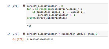
This shows that masculinity is at least not the dominating feature in determining sexual orientation. What are the groups mostly divided on then, if not for orientation? Well, aside from one cluster being more masculine than the other, the most significant cluster differences occur at index 3 (0.316 vs 0.930) and index 9 (0.172 vs 0.757). A ¼ point difference also occurs in index 10 (0.490 vs 0.752).

• Index 3 - How often do you cry?
• Index 9 - How often do you feel lonely or isolated?
• Index 10 - How often do you a physical fight with another person?

The less-masculine group, with a 0.316, cries much more than the 0.930 from the masculine group, the difference being an average participant response of ‘Sometimes’’ to the ‘Never’. The less masculine cluster also cries a lot more, with an average response of about ‘Often’ to ‘’Rarely, but open to it. Finally, the second masculine group is a bit more aggressive physically, with an average response of “Sometimes” vs “Rarely”. The fact that the columns (sexual relationships with men/women) that were most influential in determining orientation barely changes between the 2 clusters (about a 0.11 difference in each) shows that the non-masculine group is slightly more likely to get into sexual relations with other men and slightly less likely to get in relations with women.

Conclusion

This was a very satisfying project to do, as I had known nothing about ML algorithms and how conclusions came to be beforehand! I also learned a lot about using sklearn and matplotlib libraries. It was also a lot of fun going through different datasets, and letting my mind wander curiously about what things I might be able to deduce! It’s something I will be doing more soon. I also learned a lot from my mistakes, so hopefully the next time I tackle data will be done more elegantly.